Nested Fitting

Warning

This section is under construction. The content is incomplete and may still contain errors. We are working on it and will update it soon.

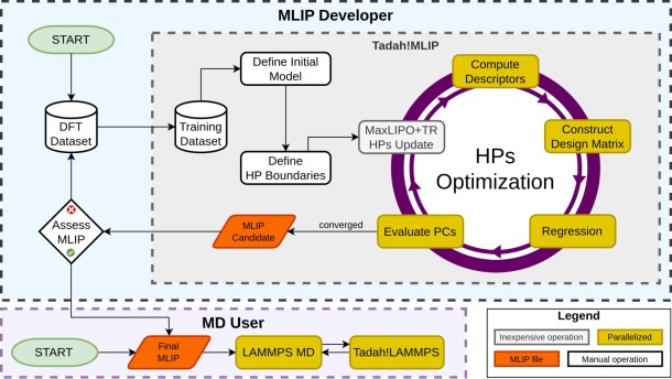
Nested Fitting Procedure — Workflow of the nested fitting procedure: the outer optimizer proposes new hyperparameters, the model is retrained, and each trial potential is validated against performance constraints that feed back into the global loss.

Nested fitting is Tadah!MLIP’s automated, two-level fitting workflow:

inner loop – ordinary regression that determines the learned parameters \(\mathbf w\) for a fixed model definition;
outer loop – a global optimizer that samples from the search space constraints (SSH), retrains the model, and judges the result against user-defined performance constraints (PC).

Letting a computer search the hyperparameter space helps to

escape the “good on the validation set, unstable in MD” trap;
trade accuracy for speed (or vice versa) in a reproducible way;
fold real-world performance constraints—elastic constants, phase stability, surface energies, …—directly into the loss function.

This page gives the necessary background and demonstrates how to set up Tadah!MLIP for nested fitting.

Background

A traditional MLIP workflow stops once regression converges on a training/validation split. Unfortunately, a potential that interpolates perfectly may still

disintegrate during an MD run
produce an incorrect equation of state
predict the wrong ground-state crystal
extrapolate poorly beyond the training set

Usual remedies, such as manual hyperparameter tuning or enlarging the training set, are both tedious and not guaranteed to succeed.

Nested fitting tackles the problem by measuring emergent properties during the fit. Each trial potential is dropped into a short LAMMPS run; the resulting quantities are compared to their targets and the discrepancy contributes to a global loss

\[L_{\text{total}} = \sum_{i} w_i\; \mathcal L_i\!\bigl(|y_i-\hat y_i|\bigr),\]

where \(w_i\) is the user-supplied weight, \(y_i\) the target, \(\hat y_i\) the prediction, and \(\mathcal L_i\) one of the built-in loss functions (L1, L2, Huber, Tukey, …).

The outer optimizer explores the hyperparameter space \(\Theta\) declared with the OPTIM directive:

\[\theta^\star = \operatorname*{arg\,min}_{\theta\in\Theta} L_{\text{total}}(\theta).\]

Because the model is retrained for every candidate \(\theta\), the procedure is computationally expensive but also powerful: it can expose regions of hyperparameter space that yield stable, accurate, and fast potentials. However, it is not a silver bullet: Success still depends on sensible choices of performance constraints and search space limits.

Quick Start

Nested fitting requires a configuration file that defines the inital model (the same file as for regular training), a validation file (simple list of datasets to validate against) and a hpo targets file that defines the outer-loop. The command to run the nested fitting is:

tadah hpo --config <FILE> --hpotarget <FILE> --validation <FILE>

See Example 2 - Basics: Nested Fitting Procedure for the simple example of nested fitting.

More examples will be added in the future. In the meantime, you can contact us for help with setting up nested fitting for your specific use case.

Manual

This manual covers the content of the configuration file format which is used to drive the nested fitting procedure. As well as some general information about the nested fitting procedure.

In general the following steps are required to run the nested fitting procedure:

Define the initial model in the training configuration file.

List validation dataset(s) in the validation file using dbfile keyword.

Define the nested fitting configuration file with the following blocks:

LOSS to define the default loss function

OPTIMIZER block to define the outer optimizer

OPTIM line(s) to define the SSH

PC_<TYPE> line(s) to define the PC:

PC_ERMSE for validation RMSE of energies (see Performance constraints for more)

PC_LAMMPS line(s) to define the physics-informed performance constraints

Loss functions

The keyword LOSS is used to define the default loss function for the nested fitting procedure. Individual PC_LAMMPS simulations can override it.

LOSS <Name> [<extra params>]

The currently supported loss functions are:

Name	Extra params	Comment
`L1`	—	\(\|x\|\)
`L2`	—	\(x^2\)
`HUBER`	`δ`	quadratically near zero, linear beyond δ
`TUKEY`	`c`	redescending, zero influence for \|x\|>c
`LOG_COSH`	—	smooth alternative to L1
`RMSLE`	—	log-scaled L2 (non-negative targets)

Choosing the optimizer

The optimizer for the outer loop is specified in the nested fitting configuration file. The optimizer could be either global, local, or a hybrid of the two. The latter case is only supported by a handful of optimizers.

Tadah!MLIP supports optimizers from the following libraries:

NLOPT https://nlopt.readthedocs.io We aim to support all NLOPT algorithms which do not require analytical derivatives, i.e. all algorithms which names begin with either GN_ or LN_. See the NLOPT documentation
Dlib http://dlib.net * Local numerical optimizers (BFGS, LBFGS, CG, BOBYQA) [Work in progress…] * Global MaxLIPO+TR aka Global Function Search (GFS)
Tadah!MLIP provides basic random search and grid search optimizers.

The optimizer is specified in the OPTIMIZER block of the nested fitting configuration file.

OPTIMIZER
  <key> <value>
  ...
ENDOPTIMIZER

If an optimizer is a hybrid of global and local, the nested LOCAL block must be specified. The local block follows the same syntax as the global block, but it is used to configure the local optimizer that will be used for the local search.

OPTIMIZER
  <key> <value> ...
  ...
  LOCAL
    <key> <value> ...
    ...
  ENDLOCAL
ENDOPTIMIZER

Note that usually optimizers support only a subset of the keys listed below.

key [type]	description [available options]
`LIB` [string]	name of the optimization library [`DLIB`, `NLOPT`, `TADAH`]
`ALGO` [string]	name of the algorithm from the selected library (see below)
`MAXEVAL` [uint]	maximum number of evaluations of the loss function
`MAXTIME` [uint]	maximum time in seconds to run the optimizer
`STOPVAL` [uint]	stop the optimization when the loss is below this value
`FTOL_REL` [float]	relative tolerance for the loss function
`FTOL_ABS` [float]	absolute tolerance for the loss function
`XTOL_REL` [float]	relative tolerance for the hyperparameters
`XTOL_ABS` [float]	absolute tolerance for the hyperparameters
`POPULATION` [uint]	number of individuals in the population (for population-based optimizers)
`STEP` [uint]	step size for the optimizer
`SEED` [uint]	random seed for the optimizer (default: current time)
`VECTOR_ARR` [uint]	storege required by some NLOPT algorithms
`THREADS` [uint]	number of threads for the Dlip::MaxLIPO+TR optimizer (default: 1)
`PARAM` [string float]	generic key value pair for passing additional parameters to the optimizer
`LOG_HP` [float]	threshold for the log-scaling of the search space (experimental)

LIB	ALGO (algorithms from the selected library)
`TADAH`	`RANDOM`, `GRID`
`NLOPT`	`GN_DIRECT_L`, `GN_CRS2_LM`, `G_MLSL_LDS`, … and many more see NLOP docs
`DLIB`	`BFGS`, `LBFGS`, `CG`, `BOBYQA`, `GFS` (MaxLIPO+TR) [work in progress…]

Search space constraints

The search space constraints are defined in the nested fitting configuration file using the OPTIM directive. The OPTIM lines specify the hyperparameters that the outer optimizer will explore. Each OPTIM refers to a single KEY from a configuration file which defines the initial model, (config.train), which is then treated as an optimisation variable.

Since KEY can contain multiple values, the OPTIM lines can also specify indices to select a subset of the values. The OPTIM line can be repeated for the same KEY in case you want to supply different low and high bounds for different indices.

OPTIM syntax:

OPTIM <KEY> (indices) <low> <high>

indices must be specified in the brackets (indices...) and follow the order in the config file which defines the initial model. Indices can be comma-separated lists, ranges a-b or strides a-b:s (e.g. (1,4,7-10:2)). Indices start from 1. <low and <high> are the floating point numbers for the lower and upper bounds.

Performance constraints

The simplest performance constraints are computed for energies, forces and stresses with the mean absolute error (MAE), root-mean-squared error (RMSE) and the coefficient of determination (R²). They are evaluated on the validation set. These constraints use the default Loss functions selected in the nested fitting configuration file with the LOSS keyword.

Currently available built-ins are

Energy
PC_ERMSE PC_ErRMSE PC_MAE PC_ERSQ
Force
PC_FRMSE
Stress
PC_SRMSE

Physical constraints

Physics-informed performance constraints are introduced with the PC_LAMMPS directive in the nested fitting configuration file. Tadah!MLIP uses LAMMPS as the work-horse that turns a trial potential into the macroscopic numbers we care about; each PC_LAMMPS launches a separate LAMMPS run.

Example

PC_LAMMPS --script in.mysim \
          --varloss myVar       0   100 \
          --varloss myOtherVar 145  10

in.mysim is a regular LAMMPS input script that defines one or more equal-style variables. --varloss myVar 0 100 tells Tadah! to include the variable myVar in the global loss with target 0 and weight 100. If no loss type is given, the default LOSS from the configuration file is used; you can override it for an individual variable by appending the loss name and its parameters.

A long PC_LAMMPS line may be split with a trailing back-slash (\) for readability.

Required options

--script <file>: LAMMPS input file containing the variable definitions.
--varloss <name> <target> <weight> [loss-type p₁ p₂ …]: Evaluate loss for this variable and target and add it to the total loss with the given weight. Optional extra tokens pick a specific loss for that variable. Variable varloss must be defined in the LAMMPS script. The value is read from the LAMMPS at the end of the run.

Additional options

--invar <name> <value>: Inject a variable (equivalent to LAMMPS’ -var), allowing the same script to be reused for several structures or pressures.
--outvar <name>: Record the variable in outvar.tadah without affecting the loss—useful for diagnostic plots.
--failscore <value>: Override the global FAILSCORE. If LAMMPS crashes or the loss exceeds this value, the optimiser receives FAILSCORE for that evaluation.

Output files

Unless you change it with OUTDIR [work in progress…] every artefact produced by the outer optimiser is written to the directory in which you started ``tadah hpo``. Five groups of files are created:

Each file begins with a header line that starts with # and describes the columns. One line per iteration. First column is always step number.

File	Columns
`loss.tadah`	Wall-time, all individual loss terms followed by total loss.
`params.tadah`	The current hyperparameter vector in the order defined by your `OPTIM` lines.
`outvar.tadah`	Additional variables requested with `--outvar` plus all variables used in `--varloss`.

The rate of logging is controlled by

OUTPUT N: write a new line every N iterations (default: 10).

Whenever a new minimum of the global loss is found the corresponding rows are copied to companion files:

best_loss.tadah
best_params.tadah
best_outvar.tadah

These contain one single line: the best result so far. Use them to monitor progress in real time without parsing the full history.

BOUTPUT N: write a new line every N iterations (default: 1).

The currest best potential is always saved to best_pot.tadah.

The trained potential itself can be archived automatically.

DUMP <N> <DIR>: Save every trial potential every N iterations to DIR. Files are named pot_<iter>.tadah. The directory is created if needed. Set N = 0 to disable (default).
BDUMP <N> <DIR>: Same as DUMP but only for improvements of the best potential. Useful when you care only about the Pareto front.

Large optimisation runs can generate thousands of potentials. Keep an eye on disk usage when enabling DUMP.
The log files are plain text and append-only. They can be tailed while the optimisation is running:
```
tail -f loss.tadah
```
Each row in params.tadah matches the order of the OPTIM directives exactly. This makes it straightforward to resume a run or replay a specific parameter set with tadah train.

Performance & parallelism

Tadah!MLIP comes in two flavours, and the parallel strategy you can exploit depends on which one you compiled.

Inner loop – regression and descriptor evaluation are OpenMP parallel. Set the number of threads in the usual way:
```
export OMP_NUM_THREADS=<n>
```
Outer loop – some optimisers can evaluate several hyper-parameter sets concurrently. Control this with the THREADS key in the OPTIMIZER block (currently supported by Dlib MaxLIPO+TR).

Rule of thumb:
```
THREADS × OMP_NUM_THREADS  ≤  number of physical cores
```
Exceeding this limit will not crash the run, but the OS will oversubscribe cores and overall performance will drop.
LAMMPS runs – every PC_LAMMPS script is executed with a serial LAMMPS binary; Tadah!MLIP will attempt to run multiple of them in parallel, each on a separate core (max OMP_NUM_THREADS).

The MPI variant parallelises the inner regression across all ranks (host–client pattern). It must be linked against the MPI version of LAMMPS. Each LAMMPS calculation is spawned independently from the main communicator:

--ncpu <m>: on a PC_LAMMPS line requests that m ranks form a mini-MPI world and execute the script. Several PC_LAMMPS lines may run side-by-side, each with its own --ncpu value. The sum of all requested ranks must not exceed available ranks – 1 (one rank is reserved for the host).

Note

The MPI launcher is functional but still experimental; improved error handling and dynamic load balancing are in development.

Example:

srun -n 64 tadah hpo …          # 64 MPI ranks available
…
PC_LAMMPS --script in.elastic --ncpu 8 …
                                 # spawns mpirun -n 8 lammps …

For inexpensive models you usually gain more by increasing THREADS than by adding OpenMP threads—context-switch overhead is lower.
For very large training sets the regression dominates; in that case set THREADS = 1 and devote the cores to OpenMP (desktop build) or MPI.
Measure, do not guess: a few short test runs sweeping OMP_NUM_THREADS and THREADS over {1, 2, 4, …} will quickly reveal the sweet spot on your machine.